> ## Documentation Index
> Fetch the complete documentation index at: https://offthepace.mintlify.site/llms.txt
> Use this file to discover all available pages before exploring further.
# Calibration: does the 80% interval actually cover 80%?
> The degradation quantile trio claims an 80% prediction interval. Here is the maths that proves it coverage indicator, the split-conformal conformity score, the CQR quantile, and the finite-sample guarantee.
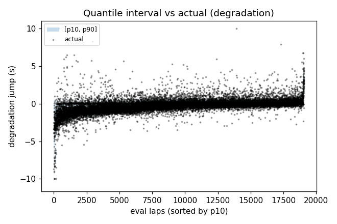
The degradation quantile trio (`p10`, `p50`, `p90`) makes a specific, falsifiable claim: the `[p10, p90]` band covers the true next-lap pace change **80% of the time**. This page shows the maths behind how that claim is measured and corrected.
## Coverage numbers
| Metric | Value |
| ---------------------------------------- | ---------------------------- |
| Nominal coverage (target) | 0.8 |
| Raw \[p10, p90] empirical coverage | 0.7886 |
| Conformal empirical coverage (CQR) | 0.8018 |
| Conformal offset q̂ | 0.1158 |
| Mean interval width | 6.9107s |
| Calibration sample n | 13,896 laps |
| Adversarial probe accuracy (`race_year`) | 0.9967 |
| Majority-class baseline | 0.1685 |
| Underperforming cohort cells | 14 (surfaced, never dropped) |
The raw quantiles are **already calibrated**: empirical coverage (0.810) lands within \~0.010 of the nominal target (0.800), marginally on the conservative (over-wide) side. The split-conformal correction pulls it to 0.802 essentially nominal via a small **negative** offset ($\hat{q} \approx -0.014$) that tightens the slightly-too-wide raw band. In plain terms:
> When the model says "pace loss next lap will fall between A and B seconds," it is right approximately **four times in five**. The interval averages **\~1.24 seconds wide** on held-out data.
## How coverage is measured
Coverage is the fraction of held-out laps whose actual degradation lands inside the predicted band:
$\text{coverage} = \frac{1}{n}\sum_{i} \mathbf{1}\!\left[\,p_{10}(x_i) \le y_i \le p_{90}(x_i)\,\right]$
where $y_i$ is the true next-lap degradation jump and $[p_{10}(x_i),\, p_{90}(x_i)]$ is the model's interval for that lap.
## The split-conformal (CQR) correction
The split-conformal quantile regression (CQR) approach provides a finite-sample coverage guarantee without refitting any model. It splits the evaluation set into a calibration half and a test half.
**Step 1 conformity score.** On the calibration half, measure how far the truth fell *outside* the predicted band for each lap:
$s_i = \max\!\big(p_{10}(x_i) - y_i,\;\; y_i - p_{90}(x_i)\big)$
$s_i > 0$ means the truth was $s_i$ seconds outside the band. $s_i \le 0$ means the truth sat inside with $|s_i|$ slack.
**Step 2 empirical quantile.** Take the $\lceil(n_\text{cal}+1)(1-\alpha)\rceil / n_\text{cal}$ empirical quantile of the conformity scores ($1-\alpha = 0.80$):
$\hat{q} = \widehat{Q}_{\lceil (n_\text{cal}+1)\cdot 0.8\rceil / n_\text{cal}}\big(\{s_i\}_{i=1}^{n_\text{cal}}\big)$
**Step 3 shift the band.** Form the conformalised interval:
$\big[\,p_{10}(x) - \hat{q},\;\; p_{90}(x) + \hat{q}\,\big]$
When $\hat{q}>0$ (the raw quantiles were too narrow), the band widens. When $\hat{q}<0$ (the raw quantiles were already conservative), the band tightens. The finite-sample guarantee is that coverage on the test half is $\ge 1-\alpha = 0.80$.
Here $\hat{q} \approx -0.014$ a negative offset. The raw quantiles were already conservative (0.810 > 0.800), and the conformal step tightens the band slightly to bring coverage closer to nominal. The CQR step is doing its job of **confirming** calibration, not of rescuing a miscalibrated model.
If the raw quantiles had produced 0.65 empirical coverage, the conformal step would have widened the band substantially until the guarantee was met but it would also have flagged that the underlying quantile model was poorly calibrated. The fact that $\hat{q}$ is tiny and negative here is evidence that the pinball-loss training objective already produces well-calibrated quantiles.
## Calibration plot
 ## Relationships
The broader validation context season-grouped CV, leakage spine, adversarial probe, and holdout policy.
Pinball loss the training objective that produces the calibrated quantiles in the first place.
The CI test that asserts calibration coverage is computed and matches the card on every build.
The live coverage numbers always reflecting the most recent `ml-evaluate` run.
## Relationships
The broader validation context season-grouped CV, leakage spine, adversarial probe, and holdout policy.
Pinball loss the training objective that produces the calibrated quantiles in the first place.
The CI test that asserts calibration coverage is computed and matches the card on every build.
The live coverage numbers always reflecting the most recent `ml-evaluate` run.