> ## Documentation Index
> Fetch the complete documentation index at: https://offthepace.mintlify.site/llms.txt
> Use this file to discover all available pages before exploring further.
# Five XGBoost tyre prediction models and their metrics
> Degradation quantile trio, cliff classifier, and stint-life regressor five XGBoost models, every one beating a per-cohort baseline, with full metrics.
The 33-feature input matrix, encoding, the three targets, and the dataset fingerprint.
The 9-dimensional Optuna search, CV selection, and full refit.
Off The Pace trains five XGBoost models on the same per-lap feature matrix and holds every one to the same standard: beat a strong, honest per-cohort baseline not just chance. All five pass that gate, and the numbers below are the proof.
The shipped parameters come from the canonical `make ml-tune` search (50+ trials, season folds, full data), stored per target in `ml/models/_best_params.json`. `make ml-retrain` refits at those parameters without re-searching, which is how a mart change ships without paying for a fresh search. A target whose data has moved should eventually be re-tuned, not only refit.
## Headline results
| Model | Kind | Metric | CV | Eval (2024) | Baseline | Beats |
| --------------------------- | -------------- | ------------ | ------ | ----------- | -------- | ----- |
| `degradation_regressor_p10` | quantile | pinball | 0.6042 | 0.5320 | 1.4644 | ✅ |
| `degradation_regressor_p50` | quantile | pinball | 1.1708 | 1.0468 | 2.1777 | ✅ |
| `degradation_regressor_p90` | quantile | pinball | 0.6434 | 0.5785 | 0.8908 | ✅ |
| `cliff_classifier` | classification | macro\_f1 | 0.3717 | 0.3719 | 0.2187 | ✅ |
| `stint_life_regressor` | survival | aft\_nloglik | 2.1481 | 1.9878 | 2.1869 | ✅ |
*CV is the season-grouped `TimeSeriesSplit` mean across five folds. Eval is the final fold (2024), standing in as a holdout until 2025 data ingests. See [Validation](/ml/validation) for the full CV scheme and the per-cohort baselines. For individual model hyperparameters and per-cohort breakdowns, see the [Model Reference](/reference/ml/degradation-model).*
***
## How the models learn
All five models are gradient-boosted decision-tree ensembles (XGBoost). A prediction is an additive sum of $K$ regression trees, built greedily one residual-correcting tree at a time:
$\hat{y}_i = \sum_{k=1}^{K} f_k(x_i), \qquad f_k \in \mathcal{F}$
where $\mathcal{F}$ is the space of CART trees and $K$ is `n_estimators`. Training minimises a regularised objective that trades goodness-of-fit against tree complexity:
$\mathcal{L} = \sum_i \ell\!\left(y_i,\, \hat{y}_i\right) \;+\; \sum_{k=1}^{K}\Omega(f_k), \qquad \Omega(f) = \gamma\,T \;+\; \tfrac{1}{2}\lambda\lVert w\rVert^2 \;+\; \alpha\lVert w\rVert_1$
$T$ is a tree's leaf count and $w$ its leaf weights. The three regularisation strengths map directly to the tuned hyperparameters in the [model card](/reference/ml/degradation-model): $\gamma$ = `gamma` (minimum split-loss), $\lambda$ = `reg_lambda` (L2), $\alpha$ = `reg_alpha` (L1). The **only** thing that differs between the five models is the per-row loss $\ell$ the objective function below.
***
## Objective functions
### Pinball loss (the quantile trio)
The three degradation regressors minimise the **pinball (quantile) loss** at $\alpha \in \{0.1,\, 0.5,\, 0.9\}$ (`reg:quantileerror`). For a residual $u = y - \hat{y}$:
$\ell_\alpha(y, \hat{y}) = \max\!\big(\alpha\,u,\;(\alpha-1)\,u\big) = \begin{cases} \alpha\,u & u \ge 0 \\[2pt] (\alpha-1)\,u & u < 0 \end{cases}$
The asymmetry is the entire mechanism. At $\alpha = 0.9$ an under-prediction ($u>0$) is penalised nine times harder than an over-prediction, so the fitted surface is pushed up to the 90th percentile; at $\alpha = 0.1$ the penalty flips and the surface settles at the 10th. At $\alpha = 0.5$ the loss is symmetric and reduces to mean absolute error, recovering the median. This is why $\alpha=0.1$ gives the optimistic bound, $\alpha=0.9$ the pessimistic one, and the three together form the $[p_{10}, p_{90}]$ interval.
### Censored AFT likelihood (stint life)
The stint-life model is a survival fit, not a regression. **46.2% of its training rows are right-censored**: on a driver's last stint of a race the tyre is still on the car when the flag falls, so the life we observe is a *lower bound*, not the life the tyre had. Squared error against that bound trains the model to predict when the pit wall stopped, which is not the question.
It therefore minimises the accelerated-failure-time negative log-likelihood (`survival:aft`) over an interval label, fitting $\log(y + 1) \sim \mathcal{N}(\mu, \sigma)$ so that $y+1$ is log-normal:
$\ell(y,\mu) = \begin{cases} -\log \phi\!\left(\tfrac{\log t - \mu}{\sigma}\right) + \log(t\sigma) & \text{uncensored, } t = y+1 \\[4pt] -\log\!\left[1 - \Phi\!\left(\tfrac{\log t - \mu}{\sigma}\right)\right] & \text{censored} \end{cases}$
The two branches are the whole mechanism. An uncensored row is scored on the *density* at the life we saw; a censored row is scored on the *survival function*, the probability of lasting at least that long. Predicting more life than we observed is nearly free on a censored row and expensive on an uncensored one, which is exactly the asymmetry the data has.
The $+1$ shift exists because $\log 0$ is $-\infty$ and 2,264 training rows have zero remaining life 2,236 of them (98.8%) censored, i.e. final laps of final stints. It is subtracted back at prediction time.
The fitted scale $\sigma = 0.8$ was swept at the production hyperparameters (CV NLL 2.237 at $\sigma=0.5$, **2.0905 at $\sigma=0.8$**, 2.115 at $\sigma=1.0$ an interior optimum). Because the fit is log-normal, that one number yields the whole distribution: the median is $e^{\mu}$ and any percentile is $e^{\mu + \sigma \Phi^{-1}(q)}$, which is what lets the app render a $[p_{10}, p_{90}]$ band from a single model output.
Predictions are clipped at $\ge 0$: a stint cannot have a negative number of laps remaining.
Stint life is **never** reported as a pooled RMSE. Scoring only the uncensored stints measures the pit wall's selection rather than the model an artefact that once produced an apparent "+12.4% improvement" from simply discarding censored rows. The headline is the censored NLL, with the C-index beside it and the two populations reported separately.
### Softprob with balanced class weights (the cliff classifier)
The cliff classifier minimises multiclass cross-entropy over a softmax (`multi:softprob`) across the four `laps_until_cliff_class` buckets. Because the classes are imbalanced (≈76% `none_in_stint`), each row is weighted inversely to its class frequency sklearn's *balanced* scheme:
$w_c = \frac{n}{C \cdot n_c}$
for a class $c$ with $n_c$ members, $C = 4$ classes, and $n$ rows in total. A rare `0_to_2` lap therefore carries several times the gradient of a common `none_in_stint` lap, which is what keeps the high-value imminent-cliff windows from being optimised away by the majority class.
### Inverse-censoring survival weights (the quantile trio)
The quantile regressors carry one further weight on top of the loss: an **inverse-probability-of-censoring (IPW) survival weight** $w_i = 1 / \hat{S}(t_i)$, the reciprocal of the probability that stint $i$ survived (avoided being pitted) to its current lap $t_i$. Without it, the high-`lap_in_stint` tail is dominated by the durable stints that happened to run long, and the genuinely degraded stints that were pitted early are under-counted biasing the predicted degradation downward exactly where the cliff matters most.
***
## Degradation quantile trio
The three quantile regressors share the pinball loss objective (`reg:quantileerror`) but target different quantiles of `next_lap_degradation_jump_s` the fuel-corrected pace change the **next** lap will show, measured in seconds.
**What this tells you:** the **p50 model gives you the median expected pace loss next lap** the single best guess at how much time this tyre will cost relative to its current pace. The **p10 model is the optimistic bound**: nine times out of ten, real pace loss will be worse than this. The **p90 model is the pessimistic bound**: nine times out of ten, real pace loss will be better than this. Together, `[p10, p90]` forms an 80% prediction interval that honestly brackets the next lap four times in five see [Validation](/ml/validation) for the coverage numbers.
**When to rely on it:** the interval is most useful when you want to compare tyre risk between two stints or set a pit-window trigger. A narrow band means the tyre's behaviour is predictable; a wide band flags genuine uncertainty.
**Limits:** the target is legitimately **negative roughly 44% of the time** a tyre coming into its working window, or recovering after an out-lap, genuinely gains pace. The model captures this, but intervals on the first two or three laps of a stint are wider as the tyre is still warming.
The quantile outputs are always monotone p10 ≤ p50 ≤ p90 so crossed intervals never reach the UI. Each regressor's baseline is the honest naive answer in the same `(compound, circuit, age-bucket)` cells: the cell group-mean for p50, the empirical 10th/90th percentile for p10/p90. Beating a per-cell empirical percentile means the model adds real signal beyond "what usually happens here."
***
## Cliff classifier
The cliff classifier is a 4-class model over `laps_until_cliff_class`, trained with `multi:softprob` and **balanced class weights** to keep the rare imminent-cliff windows from being drowned out by `none_in_stint`, which carries roughly three quarters of all laps.
**What this tells you:** where the tyre sits relative to a cliff. The four classes map directly to how urgent the strategy call is:
| Class | Meaning | Approx. share |
| --------------- | -------------------------------------------------------- | ------------- |
| `0_to_2` | Cliff imminent within the next two laps | \~9% |
| `3_to_5` | Cliff approaching three to five laps away | \~7% |
| `6_plus` | Cliff six or more laps away, but still inside this stint | \~9% |
| `none_in_stint` | No crossing anywhere in the remaining stint | \~76% |
**When to rely on it:** use the classifier's output as a yellow/amber/red alert for pit-stop timing, not as a lap-precise countdown. The probability scores for each class are surfaced a high probability on `0_to_2` is a stronger signal than a marginal one.
**Limits read this.** The model's macro-F1 of 0.404 comfortably beats the majority-class prior (0.224), and the balanced weighting earns its keep on the minority imminent-cliff windows. It is still the model to be most careful with, but **not for the reason this page used to give.**
The old reading was "macro-F1 ≈ 0.40 is modest in absolute terms". That compares 0.404 against 1.0, and 1.0 is not a score anything could reach on this label: laps inside a stint share a compound, a car, a circuit, a fuel load and a driver, so a large part of the class is fixed before the lap is run. Measured against an oracle that is handed the stint id and nothing else, the model reaches **114% of that ceiling** it is not the ceiling that is holding it back. The real limit is upstream: `laps_until_cliff_class` is a first-crossing scan over a polynomial cliff curve that is unbounded, so part of what the model is being asked to reproduce is an artefact of the label's construction rather than a fact about the tyre.
Treat `0_to_2` calls as a strong prompt to look at the degradation band, not a lap-precise certainty. The largest confident misses are reviewed continuously. See also [Tyre cliff](/decomposition/tyre-cliff).
`laps_until_cliff_class` is also a censored time-to-event target. `none_in_stint` is just the censored bucket, and about a quarter of training rows have fewer than six laps left in the stint, so `6_plus` is not even reachable for them. The obvious move is to fit one accelerated-failure-time model on the first-crossing lap and read the four class probabilities off the survival curve, preserving the 4-column output contract exactly. That framing is the right one for the [stint-life target](#stint-life-regressor). **Measured on this target, it loses.**
Evaluated on rows with at least 15 laps left, where all four buckets are fully observed over a fixed horizon and nothing in the metric depends on when the team actually pitted:
| Model | macro-F1 (higher better) | log-loss (lower better) |
| --------------------------------------- | ------------------------ | ----------------------- |
| multiclass `multi:softprob` | **0.3704** | 1.1503 |
| AFT to bucket probabilities, scale 0.35 | 0.2918 | 2.5485 |
| AFT to bucket probabilities, scale 0.7 | 0.3331 | 1.3009 |
| AFT to bucket probabilities, scale 0.9 | 0.3329 | 1.1350 |
| AFT to bucket probabilities, scale 2.0 | 0.2566 | **0.9593** |
The scale was swept rather than fixed at one value, so the result is a property of the framing and not of a badly chosen constant. The trade is legible: AFT buys better *calibration* at wide scales (log-loss 0.959 against 1.150) and worse *discrimination* everywhere. Macro-F1 never reaches the multiclass model, and at the log-loss optimum the AFT model has collapsed to predicting the base rate. Macro-F1 is this target's headline metric, so the multiclass model keeps the slot. Measured 2026-08-23.
***
## Stint-life regressor
The stint-life model predicts `remaining_stint_life_laps` a synthesised, non-negative count of usable laps remaining in the stint as an accelerated-failure-time survival fit (`survival:aft`, log-normal, clipped ≥ 0).
**What this tells you:** this is the number behind the strategy view's "this set has approximately N laps left" readout. It integrates tyre age, thermal load, and compound character into a median, and because the fit is log-normal it also yields the $[p_{10}, p_{90}]$ band shown beside it.
**When to rely on it:** read the band, not the median alone. The gauge colours by $p_{10}$ rather than the median, because "how soon could this tyre be done" is the decision the colour is used for, and the pessimistic end is the honest answer to it. The estimate tightens as the stint progresses.
**Why it is not an RMSE:** almost half the training rows are censored, and a point error against a lower bound is not an error. The model is scored on the censored likelihood, with the C-index as the ranking check and the censored and uncensored populations reported apart. The blind-test scoreboard shows both columns and never averages them.
**Limits:** its baseline is **knowingly near-oracle** it uses the true final stint length the model is explicitly forbidden to see yet the model still wins under the censored likelihood. Cohort losses on specific circuits are recorded openly rather than dropped.
***
## Tuning and refit
Each model is tuned with Optuna (`TPESampler` + `MedianPruner`, seeded), then refit on the full training set. Cross-validation selects the hyperparameters; the complete dataset trains the shipped booster. The 9-dimensional search space and the full Steps walkthrough live on the [Tuning page](/ml/tuning).
***
## ONNX export and in-browser scoring
Every model is exported to ONNX and passes a round-trip parity test to `atol=1e-5` including a NaN-bearing sample that confirms parity holds on the \~47% of laps with a null cliff-onset prior. This export is what allows the React app to score predictions entirely client-side, with no server required. Full details on the [ONNX page](/ml/onnx).
Suppose, on lap 14 of a stint, the trio outputs **p10 = −0.05 s**, **p50 = +0.18 s**, **p90 = +0.61 s**.
* The **median** call is "next lap costs ≈ 0.18 s of pace."
* The **80% interval** is `[−0.05, +0.61]` four times in five, the real next-lap change will land in that band.
* The interval is *asymmetric and skewed positive* the downside tail (+0.61) is wider than the upside (−0.05), which is the model saying the tyre is more likely to lurch slower than faster. That asymmetry is the early warning the cliff classifier then quantifies as a class.
A symmetric band tight around zero means a settled tyre; a band that fans out on the positive side is a tyre starting to ask questions.
The decomposition already runs the linear, physics-grounded corrections each one a single coefficient per dimension. The cliff is where that approach runs out: it is an *interaction* effect ("Soft **and** lap 14 **and** six laps of dirty air **and** a hot low-grip surface"), and a linear model would need every interaction term hand-specified. Boosted trees discover the interactions that matter from the data, which is precisely the job the linear layer cannot do. The trade is interpretability, recovered post-hoc via SHAP (see [Model Reference → feature importance](/reference/ml/degradation-model#feature-importance-shap-vs-permutation)).
***
## What the p50 regressor learned
A partial-dependence plot isolates how the median-degradation model's output moves with each of its three most important features, holding the rest fixed the post-hoc interpretability the SHAP analysis quantifies.
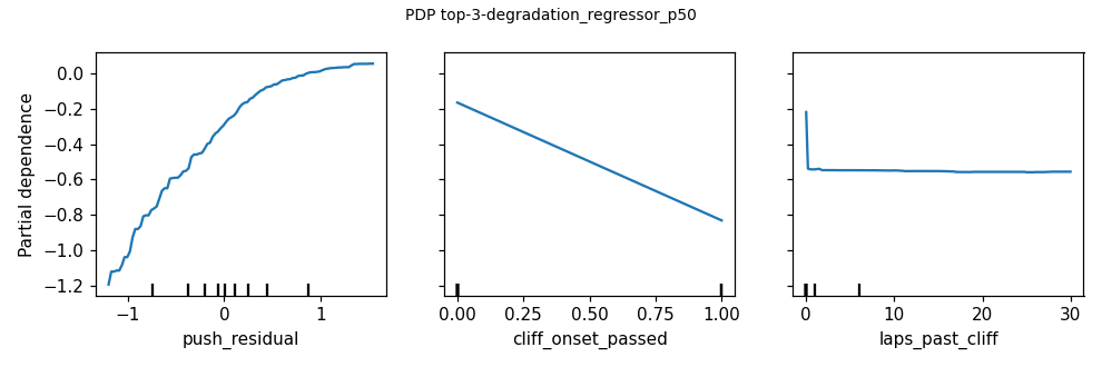 * **`push_residual`** is the dominant, near-monotone driver: the harder a lap is pushed relative to its stint, the more the model expects the *next* lap to give back.
* **`cliff_onset_passed`** (a binary flag) and **`laps_past_cliff`** move the median once the tyre crosses its modelled cliff `laps_past_cliff` saturates almost immediately, consistent with the cliff being a step change rather than a gradual slope.
See the [Model Reference](/reference/ml/degradation-model#feature-importance-shap-vs-permutation) for the full SHAP-vs-permutation importance ranking behind this selection.
* **`push_residual`** is the dominant, near-monotone driver: the harder a lap is pushed relative to its stint, the more the model expects the *next* lap to give back.
* **`cliff_onset_passed`** (a binary flag) and **`laps_past_cliff`** move the median once the tyre crosses its modelled cliff `laps_past_cliff` saturates almost immediately, consistent with the cliff being a step change rather than a gradual slope.
See the [Model Reference](/reference/ml/degradation-model#feature-importance-shap-vs-permutation) for the full SHAP-vs-permutation importance ranking behind this selection.