> ## Documentation Index
> Fetch the complete documentation index at: https://offthepace.mintlify.site/llms.txt
> Use this file to discover all available pages before exploring further.
# Hyperparameter tuning: Optuna search, CV selection, and full refit
> How Optuna TPESampler explores the 9-dimensional hyperparameter space for each of the five models, selects on season-grouped CV, and then refits on the full training set.
Every model in the pipeline is tuned by Optuna before its final fit. Tuning and training use deliberately separate data that separation is what keeps the headline CV metrics honest.
Optuna's `TPESampler` (seeded at `RANDOM_STATE`) proposes hyperparameter configurations from a 9-dimensional space. `MedianPruner` kills unpromising trials after each CV fold, keeping the search efficient even with 50 trials.
| Hyperparameter | Type | Range | Role in the objective |
| ------------------------ | ----------- | --------- | ------------------------------------------------------------- |
| `n_estimators` | int | 200–700 | Tree count $K$ more trees = lower bias, more variance |
| `max_depth` | int | 3–8 | Max depth per tree controls complexity |
| `learning_rate` | float (log) | 0.02–0.20 | Shrinkage per tree lower = smoother, needs more trees |
| `subsample` | float | 0.6–1.0 | Row sampling per tree regularisation via stochasticity |
| `colsample_bytree` | float | 0.6–1.0 | Column sampling per tree feature-dropout regularisation |
| `min_child_weight` | int | 1–20 | Minimum Hessian sum to make a leaf prunes fine-grained splits |
| `gamma` ($\gamma$) | float (log) | 1e-3–5.0 | Minimum split-loss directly in the regularised objective |
| `reg_lambda` ($\lambda$) | float (log) | 1e-3–5.0 | L2 leaf-weight regularisation |
| `reg_alpha` ($\alpha$) | float (log) | 1e-3–5.0 | L1 leaf-weight regularisation |
The three regularisation strengths $\gamma, \lambda, \alpha$ map directly to the terms in the XGBoost regularised objective:
$\Omega(f) = \gamma\,T \;+\; \tfrac{1}{2}\lambda\lVert w\rVert^2 \;+\; \alpha\lVert w\rVert_1$
where $T$ is the leaf count and $w$ the leaf weights. All three are searched on a log scale because their effect is multiplicative a move from 0.001 to 0.01 matters as much as a move from 1.0 to 10.0.
Each trial is evaluated by season-grouped `TimeSeriesSplit` across **five folds**. The folds respect temporal ordering future seasons never inform models of past seasons and the headline metric varies by model family:
* **Quantile trio**: mean pinball loss across folds (↓ lower is better)
* **Cliff classifier**: mean macro-F1 across folds (↑ higher is better)
* **Stint-life regressor**: mean RMSE across folds (↓ lower is better)
After the study completes, the best parameters are written to `ml/models/{target}_best_params.json`. The Optuna study is persisted to `ml/models/optuna_studies/{target}_{version}.db`, so it is resumable a rerun with `load_if_exists=True` extends the existing study rather than starting from scratch.
Once the best hyperparameters are selected, the booster is trained on the **entire training set** (all seasons except the holdout). Cross-validation selected the configuration; the complete dataset trains the shipped model.
This is the step that produces the `.bst` booster artefacts. The refit runs automatically after tuning completes `make ml-tune` chains into `ml-train` for the tuned version.
**Reduced v1 budget.** The shipped v1 parameters used a reduced tuning budget (15 trials / 3 folds / 30,000-row search subsample) for speed during initial development. The canonical `make ml-tune` (50 trials / 5 folds / full data) only improves the parameters. The beats-baseline gate holds regardless of budget.
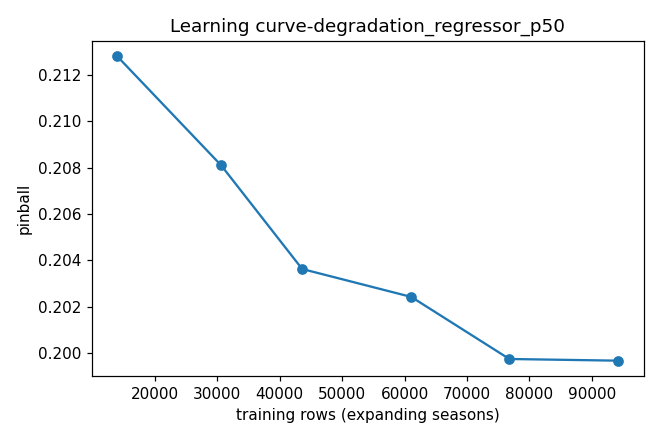 Every study is keyed by `{target}_{version}` (e.g. `cliff_classifier_v5`) so a fresh tuning run for a new version gets its own namespace without overwriting the existing study. The `TPESampler` is seeded by `RANDOM_STATE = 20260528`, so two runs with the same data and the same budget produce the same parameter sequence.
The `.db` files are SQLite they can be inspected with `optuna-dashboard` or the `scripts/inspect_trials.py` utility. CI does not run `ml-tune` (it is too slow for pull requests); it runs `ml-test` against the committed `.bst` artefacts.
## Relationships
The five objectives and why each model's loss function shapes what the tuning search is optimising.
Season-grouped CV the same scheme the tuning search uses as its objective.
The committed best-parameter values for each model, alongside the headline metrics they produce.
Where `ml-tune` sits in the full `make ml-all` DAG.
Every study is keyed by `{target}_{version}` (e.g. `cliff_classifier_v5`) so a fresh tuning run for a new version gets its own namespace without overwriting the existing study. The `TPESampler` is seeded by `RANDOM_STATE = 20260528`, so two runs with the same data and the same budget produce the same parameter sequence.
The `.db` files are SQLite they can be inspected with `optuna-dashboard` or the `scripts/inspect_trials.py` utility. CI does not run `ml-tune` (it is too slow for pull requests); it runs `ml-test` against the committed `.bst` artefacts.
## Relationships
The five objectives and why each model's loss function shapes what the tuning search is optimising.
Season-grouped CV the same scheme the tuning search uses as its objective.
The committed best-parameter values for each model, alongside the headline metrics they produce.
Where `ml-tune` sits in the full `make ml-all` DAG.